
Stock Target Price Predictor
Metis Module 4 - Machine Learning Classification
Stock predictions as a classification problem.
ABSTRACT
I developed a classification pipeline that takes in a stock’s price data from the TD Ameritrade API, transforms the data using a series of custom functions and evaluates that stock relative to a trading system known as The Strat. The classification problem is: what is the probability that a stock will hit its target price using The Strat trading system? I trained the data on five models to find the model that best predicts on the test data. The model with the best performance was a tuned Random Forest, which predicted with a .74 accuracy on the test data. I then used this model to predict stock performance for the month of September, which returned a .80 accuracy score and 80% success rate on the top five stocks with the highest probability of success.
BACKGROUND
In an attempt to find an edge in the financial markets, I searched far and wide for a profitable strategy that made sense and was consistently objective in its approach. After years as a market maker who made trades based on customer needs and my own book’s risk, I now wanted to find edge and take a proprietary approach for my own endeavors. After six months of trying different strategies and services but only finding inconsistency mitigated by risk control, I stumbled upon and reached out to a man by the name of Rob Smith. Rob, a storied stock trader and former member of the Chicago Stock Exchange, developed a unique interpretation and strategy with regard to the markets known simply as The Strat. His entire system is based on, what we know to be true, which in turn can signal why we can expect price to move, or more specifically “actionable signals quantify specific technical conditions [which causes price to move].”
Before we go deeper, I would like to provide a small section on the anatomy of a candlestick, which is integral in interpreting The Strat. Financial platforms can graph any tradeable financial product’s price. Each graph can be a simple line chart of closing prices on any time frame (time frame can mean any aggregated time period such as an hour, day, or week) or a more complex but more informative candlestick chart that displays red and green bars representative of a specific time frame. Here is an image that breaks down the anatomy of a candlestick:
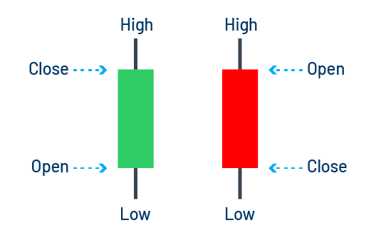
Note if a candlestick is red, that means the close of that time frame is lower than its open, which shows the product fell in price for that period. The opposite is true for a green candlestick. The top of a candlestick is the highest price the product traded for that period and the bottom is the lowest. For our purposes we will only concentrate on the high and low of each candlestick. Additionally, for this paper, we will use the words ‘candlestick’ and ‘bar’ interchangeably.
In Rob’s system he defines three scenarios:
- Scenario One: The current candlestick’s high and low does not break the high and low of the previous candlestick. This is known as a “1” bar or inside bar and represents that equilibrium has formed: buyers/sellers are not signaling new price discovery by taking out the previous candlestick’s highs or lows.
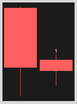
- Scenario Two: The current candlestick took out the previous candlestick’s high or low, this is known as a “2” bar and signals that buyers/seller attempted to break equilibrium and signal new price discovery.
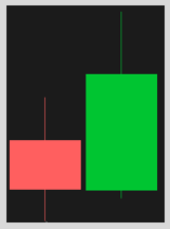
- Scenario Three: The current candlestick takes out the previous candlestick’s high and low, this is known as a “3” bar or outside bar. Three bars signal that a broadening of price has occurred (new high/low price discovery occurred in either the near or long term). Keep in mind, because buyers/sellers are willing to pay up/sell down the price of the stock, they will be willing to do it again in the future.
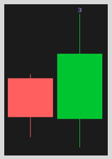
Based on these three scenarios, Rob identifies a series of combinations that attempt to take advantage of the price broadening described in Scenario Three, but in a ‘broader’ sense. If price can reverse and trade both higher and lower than the previous candlestick’s high and low, as in a Scenario Three, then price should be able to do the same but over an extended period and across multiple candlesticks as shown here:
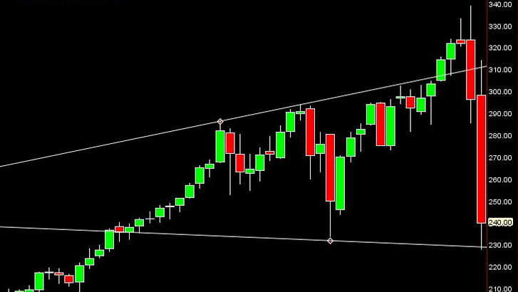
Rob calls this the broadening phenomenon and states, “everything that trades will trade in a continuous series of ‘price discovery broadening formations: PERIOD.” Because of this phenomenon, we can use the following combinations to take advantage of these regions of potential reversals or potential continuations of price.
The series of combinations identified by Rob and that I used as potential setups for this model are as follows (note: I only used ‘long’ setups or setups where the user would be buying the financial product):
- 1 scenario setup:
- Occurs when an inside bar forms and price confirms the setup by moving above the one bar, attempting to break equilibrium. Magnitude is the high of the bar that preceded the inside bar.
- 3-2 scenario setup:
- Occurs when a two bar to the downside forms after a three bar and price confirms the setup by moving above the two bar. Magnitude is the high of the three bar.
- 2-2 scenario setup:
- Occurs when a two bar to the downside forms after a two bar to the upside and price confirms the setup by moving above the two bar. Magnitude is the high of the two bar to the upside.
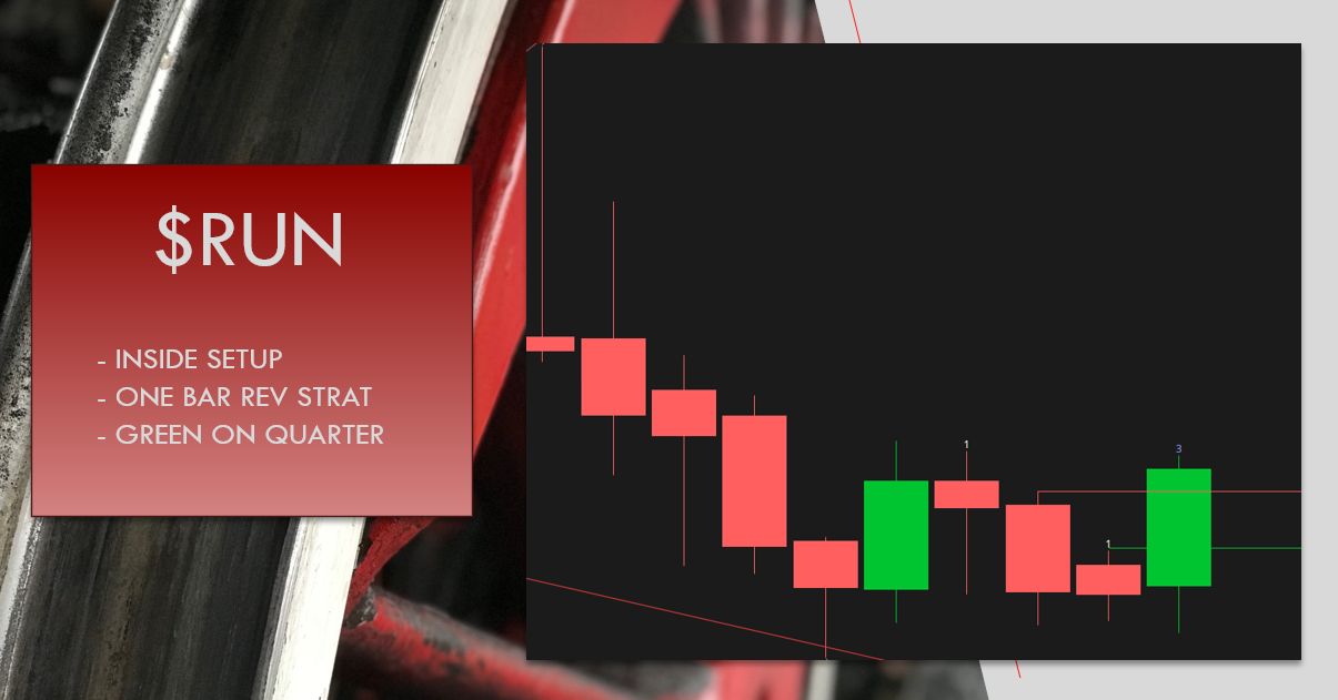
- 1-2 scenario setup also known as a “bullish 2-bar Rev Strat”:
- Occurs when a two bar to the downside forms after an inside bar and price confirms the setup by moving above the two bar. Magnitude is the high of the bar that preceded the inside candlestick.
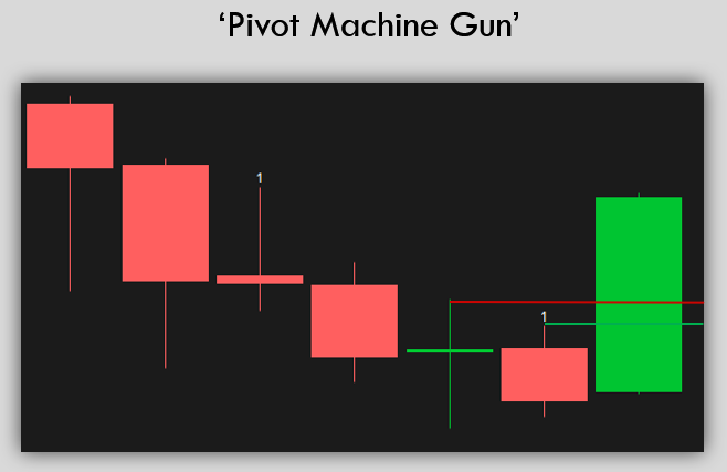
- ‘PMG’ scenario also known as “pivot machine gun”:
- Occurs when (as defined by me on the monthly) three or more bars have had consecutive lower highs and price confirms the setup by moving above the high of the previous bar. Magnitude is at least the high of the bar prior to the previous bar. If price can manage to reverse direction and take out the previous bar’s high in this scenario, buyers as well as established shorts who will need to cover (the sellers become buyers, known as a squeeze) can, in tandem, quickly move price higher.
A success in terms of these setups is if price trades at magnitude within a three-month period (my own criteria). A failure is if price trades lower than the low of the current bar at the time the setup activates before price trades at magnitude. Note, many times a setup is present, but if the setup never activates (remember price confirms the setup by moving above the previous bar) or if price gaps above the previous bar (meaning that price opens above the previous bar on either the monthly or daily time frame, then the trade was never activated and cannot be counted as a success or failure, because no trade would have been made.
BUSINESS CASE
While The Strat is objective and easily interpretable, there are layers of caveats needed for its success. As with any trading strategy there are moments when The Strat setups do not work, but typically there are a series of objective reasons why they failed. Given this, if I could engineer features that correlate to when The Strat is successful and when it is not, then I could theoretically train a classification model that consistently identifies the probability of each setup reaching its target price.
And that is exactly what I set out to do.
The Strat can work on any time frame, but for the purposes of this model, I wanted to provide users with the ability to invest with The Strat on higher time frames so that they can place orders with a predefined risk and target price, and let those orders play out without micromanaging every second. Therefore, the model I produced only makes predictions for the monthly time frame.
MATERIALS AND METHODS
DATA
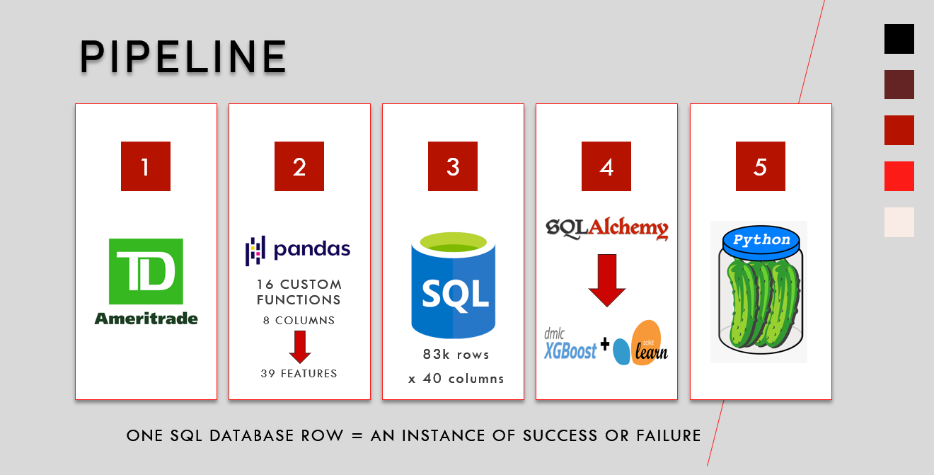
I chose to only concentrate on long setups for this model due to time constraints and complexity of coding needed to achieve such a model. I used the Python requests library to pull historical price data from the TD Ameritrade API using a list of the top 4,500 stocks with the largest market value. I then used a for loop to iterate through the list of stocks. For each request and if available, the API returned up to 20 years of data for the daily open, high, low, close, and volume of each stock in json format. I then stored the data into a data frame and used a combination of sixteen custom functions and over one hundred custom transformations within the for loop to clean the data and produce a final Pandas data frame. The for loop then appended each data frame to a SQL database for storage. The final database resulted in 83k rows and thirty-eight columns, two-thirds of which were successes, and took one hour and forty minutes to generate. Additionally, I used the same structure to pull historical data for the S&P 500 to produce additional features which a for loop then saved to a separate SQL database for storage.
To put this all into perspective, from eight columns, I was able to produce a total of thirty-nine price only specific features, meaning I pulled no financial data or any other outside data to supplement the data collection and feature engineering process.
In terms of features, examples are as simple as the year: what year did the setup activate? Or as complex as: how long has the stock been trading in the same range? Did the current bar or previous bar achieve a six-month high? Was the S&P 500 a monthly inside bar (at equilibrium) at the time the setup activated? What was the risk/reward ratio for the trade?
ASSUMPTIONS/BIAS IN THE DATA
The data used for this analysis only encompasses 4,500 stocks, missing over three thousand of the smallest market names. Furthermore, using the S&P 500 for additional features is only one metric with which to do so. A more granular approach using different indexes, ETFs, or sector/industry specific groupings would enhance model results.
RESULTS
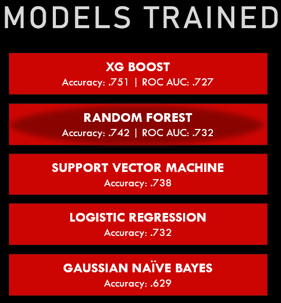
My plan of attack was to train multiple models, optimize the best models, determine the model with the highest accuracy score (how many observations, both positive and negative, were correctly classified), and then use that model to classify setups from the month of September to see how well the model predicted. I used SQL Alchemy to load my databases into a Pandas data frame. I then imported machine learning algorithms from Scikit-Learn and XG Boost for evaluation. The models I chose to evaluate (I ran all models with the same 80/20 train/test split and scaled my features) were Logistic Regression, Random Forest, XG Boost, Gaussian Naïve Bayes, and Support Vector Machine (‘SVM’). Additionally, for Logistic Regression and Random Forest I evaluated both models with a balanced class weight, but both instances performed worse than without a class weight, so I did not incorporate a balanced class weight for final evaluation.
Of the five models, Random Forest (.743) and XG Boost (.751) produced the highest accuracy scores. I then used GridSearchCV to tune Random Forest and XG Boost using customized dictionaries to test each model for their best parameter plug ins. After the completion of each GridSearchCV, I then re-ran each model with the updated parameter plug ins. Random Forest’s accuracy score got marginally better at .745 and XG Boost’s accuracy score also saw marginal gains at .753. To dig slightly deeper into each model, I then graphed an ROC AUC (Receiver Operating Characteristic Area Under the Curve) for each model against the test data, which like accuracy distinguishes between correctly classified observations, but does so at various thresholds. The ROC AUC for Random Forest was .732 which outperformed the ROC AUC for XG Boost at .727. Because I care about ranking my predictions, a higher ROC AUC is better for my use case. Therefore, I chose the tuned Random Forest model to use for my predictions.
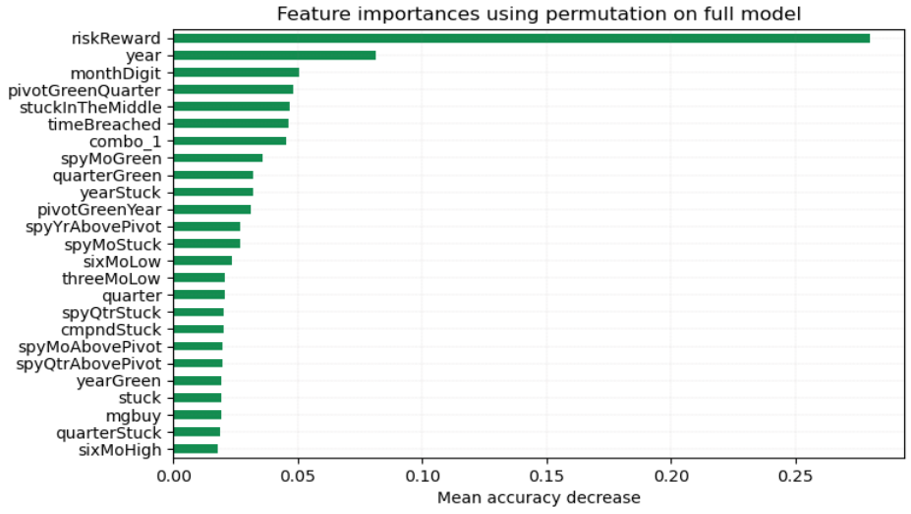
After running feature importance using permutation on the full model, the features with the most impact on the model were the risk/reward ratio, year, month, if price is stuck in the middle of the previous bar and the time of the month when price confirmed the setup by moving above the high of the previous bar (did this happen in the first half of the month or second?). Of extreme interest, risk/reward was every model’s most impactful feature, but I was able to specifically identify that it showed a negative correlation within the logistic regression model, meaning that the greater the risk, the more likely the stock was to meet its target. I used this interpretation to understand risk/reward’s impact in the Random Forest model, but I will get more into this in the conclusion.
I then pickled the tuned Random Forest model (pickled means saved) to use in a separate notebook to predict set ups for the month of September. To get the most current information, I re-pulled all stock data from the TD Ameritrade API to feed into the tuned Random Forest model. The model predicted with .80 accuracy!
The following five stocks had the highest predicted probability, shown with their results. The last column shows the money made if a user invested five thousand dollars in each stock:
| Ticker | Combo | Prediction | Percent Capture | Hit Target | Money Made | |
|---|---|---|---|---|---|---|
| 1 | TGLS | 1 | .996 | 5.1% | 1 | 255 |
| 2 | HLIT | 1 | .996 | 6.35% | 1 | 317.5 |
| 3 | OCGN | 1 | .976 | 6.9% | 1 | 345 |
| 4 | TDUP | 1 | .994 | 7% | 0 | 0 |
| 5 | RUN | 1 | .924 | 12.7% | 1 | 635 |
Of the five stocks, all met their target, and one is still working, meaning that it did not meet its target. This is an 80% success rate, BUT of the stock that is still working, in this system it still has two months to potentially hit its target, meaning that it has not failed yet.
Example: $RUN in September
CONCLUSION
While I am decently happy with the results of this model, I still have more work to do. The model, at this point, is a good starting place and provides impetus to continue its evaluation and the significance The Strat can have for its users. The most impactful feature, risk/reward, was surprising to me, but the more I consider its impact the more intuitive it seems. In practice, most individuals would want to take less risk for a higher reward, so if sellers sold a stock down in price, they are comfortable with a risk/reward that favors their position in that stock at that moment. However, if price reverses and buyers gain control and the stock rises in price against their position, just like the PMG setup, those sellers who were once comfortable and at a profit, suddenly become buyers who then work in tandem with natural buyers to accelerate the price of the stock higher. Think of it as a panicked mad rush: everything was great…now its not, emotion takes over and everyone starts buying: supply of the stock dries up and price rapidly moves higher. Surprisingly, I was expecting a specific setup to be more impactful, such as a PMG or 1-2 scenario but inside bars proved most impressive showing the simplicity of a break in price equilibrium.
IMPACT
This model lays the groundwork for a more in-depth analysis and programmatic development of The Strat for widespread use. As it stands, an individual could use this model and find success, but I need to fine-tune the model, optimize it for second-to-second evaluation, and then scale it for intensive use.
FUTURE WORK
I would like to rewrite the code used to scrape data for this model to be even more precise than just the day the stock’s price confirmed the setup. This model, for greatest accuracy needs second to second evaluation that would need to utilize parallel computing to monitor each stock relative to not only the general market at the time of execution, but also its industry. Furthermore, a trading strategy that employs risk control would be beneficial for the user, which would not allow the actual risk to exceed 5%, especially when several stocks with the highest probability of success in September had over 40% risk!
Check out the code for this project on GitHub!